Ultimate 2048 CS 175: Project in AI
Final Video Summary
Project Summary
Ultimate 2048 aims to explore and compare the efficacy of various reinforcement learning (RL) algorithms in playing 2048: a puzzle game on a 4x4 grid where tiles of equal numbers are merged to create larger tiles indefinitely. While the game can technically go on forever, successfully reaching the 2048 tile is considered winning. Tiles of values 2 and 4 appear at random in empty spaces on the grid. If the board fills up and no additional moves are possible, the game is over. As there have been a variety of previous attempts across different contexts showing the surprising difficulty of this task, our focus is to (1) find and optimize an algorithm that can learn to reach the 2048 tile, and (2) perform a comparative analysis of Policy Gradient Algorithms - more specifically, Proximal Policy Optimization (PPO) and Advantage Actor-Critic (A2C) - and Monte Carlo Tree Search (MCTS) for this game under a single, controlled setting.
The 2048 game is considerable AI/ML task because it has an enormous number of possible board configurations - an infinite amount if the game is able to infinitely progress - and success requires long-term strategies making it infeasible to use brute force methods. With the added complexity of random tiles appearing after each move, this becomes a perfect environment for reinforcement learning algorithms which can learn to make decisions under uncertain circumstances. Further, because the game’s scoring system is non-linear with points increasing more quickly as the tiles get larger, machine learning is necessary to balance the reward function and its coefficients as the game progresses.
We are using a Python implementation of the 2048 game in order to use a 2D array game state as input. Each time the Python simulation calls the currently in-use model, the model’s output consists of two parts: (1) one of four possible next moves: up, down, left, or right and (2) an array of length four with the model’s confidence in each move at that particular point in time, expressed as a probability. By conducting this experiment, we hope to discover the strengths and weaknesses of each approach which can inform future studies regarding RL for solving complex, real-world problems involving randomness, spatial reasoning, and long-term planning.
Approaches
Our approach can be broken down into the implementation and evaluation of three different AI/ML Algorithms, which we evaluate under the same success criteria. These models were selected because of their documented strengths in solving similar tasks [1-5], and refined through the recommendations of Professor Fox in our initial proposal meeting. We also implemented a baseline model to serve as a point of comparison.
Baseline
Our baseline model simply selects a random move (up, down, left, or right) for each turn. This strategy tends to succeed early in the game when the board is fairly empty and tiles’ values are small. However, as the game progresses, random moves do not create any order on the board and thus fails. Therefore, this is a reliable baseline to check that our models are using long-term planning and reaching success in later stages of the game.
Monte Carlo Tree Search (MCTS)
Monte Carlo Tree Search is a search algorithm that balances exploration (trying new actions to discover long-term strategies) and exploitation (choosing the best-known action based on past experiences). The process follows 4 main steps: selection, expansion, simulation, and backpropagation. For 2048, MCTS constructs a search tree where nodes represent game states, and edges represent moves (up, down, left, right) linking those states. The algorithm iteratively simulates games from different starting points, updating its confidence in the different possible moves to maximize long-term success.
MCTS samples game trajectories by simulating rollouts from the current state. At each step, it selects an action using Upper Confidence Bound for Trees (UCT) [6]. This is defined as:
\[\mathcal{UCT}(s, a) = Q(s, a)+ C \sqrt{\frac{\ln \mathcal{N}(s)}{\mathcal{N}(s, a)}}\]Q(s, a) represents exploitation (favoring high rewards), and the second term encourages exploration (prioritizing less-tried actions). C is a constant to adjust the amount of exploration [6]. ln N(s) and N(s, a) represent the number of times the parent and child nodes have been visited, respectively. Further, we want to ensure that the model keeps the largest tiles in the bottom left corner to keep the board organized. To do this, we first applied a heavy penalty to actions moving right which significantly affects the board organization and a moderate penalty to actions moving up since it should be done sparingly. We also created distance functions using Manhattan distance measuring how far the largest and second-largest tiles are from the bottom left corner and the spot above the corner, respectively. Heavy penalties were applied if these distances grew. We did not implement a penalty for the third-largest tile as this restricted the model’s moves too much, worsening its performance. Therefore, our final equation for selecting the best move from each rollout is:
\[\mathcal{UCT}(s, a) = Q(s, a) + 1.5 \sqrt{\frac{\ln N(s)}{N(s, a)}} - 120000 \cdot \mathcal{I}_{right} - 20000 \cdot \mathcal{I}_{up} - 100000 \cdot D_\text{corner} - 100000 \cdot D_\text{above corner}\]To use this model in 2048, we represent states as a 4x4 array and define actions as the 4 possible moves. The reward function incentivizes tile merging and penalizes game termination. Instead of full rollouts, which can be hundreds of moves, we limited each to have a maximum of 35 steps as increasing the number had minimal benefits. We also optimized the number of trials/simulations by finding the average score of 10 games for 10, 30, 60, 100, and 130 simulations for each rollout. We found that using 60 simulations significantly outperformed other values. Additionally, we changed the exploration-expoitation tradeoff constant from 1 to 1.5 to slightly encourage more exploration before choosing the best move [1]. The high-level pseudocode describing the flow of this algorithm is shown below.
while game is not over:
    create root node with current game state

    repeat for 60 simulations:
        start at root node
        while current node is not leaf:
            select best child using UCT(s, a)
            move to selected child

        if current node not fully expanded:
            create new child node for untried move

        simulate playout of 35 moves from node

        backpropagate rewards and visit counts for all nodes in path

    choose most visited child of root
    apply chosen move to game state
MCTS is found to significantly outperform other models in 2048 by simulating many rollouts to identify high-reward, long-term action sequences. However, this advantage comes with high computational costs. MCTS requires much more time per move than policy gradient methods, and the large tree growth relies on much more memory than other methods. In our optimal model using 60 simulations per rollout, the model only performs around 65 moves per minute compared to Proximal Policy Optimization which can perform almost 500 moves per minute. This makes it difficult to perform repeated testing as efficiently as other models, but because 2048 does not have a time limit and MCTS displays a high success rate, the computational cost is worth it. Additionally, with our penalties for making undesirable moves and creating a disorganized board, this model tends to make smart, long-term moves and does not show signs of overfitting.
Proximal Policy Optimization (PPO)
Proximal Policy Optimization is policy gradient method that combines the sample efficiency of on-policy algorithms with stable and reliable updates. PPO is known for clipping the objective function to prevent overly large policy updates, thus stabilizing training and avoiding performance drops. The core idea behind PPO is to prevent the policy update from moving too far in a single step, maintaining stable learning.
\[\mathcal{L}^{\mathrm{CLIP}}(\theta) = \mathbb{E}_t \Bigl[ \min\Bigl( r_t(\theta)\,\hat{A}_t, \,\mathrm{clip}\bigl(r_t(\theta),\,1-\epsilon,\,1+\epsilon\bigr)\,\hat{A}_t \Bigr) \Bigr]\]where $r_t(\theta) = \frac{\pi_\theta\bigl(a_t \mid s_t\bigr)}{\pi_{\theta_\mathrm{old}}!\bigl(a_t \mid s_t\bigr)}$ is the probaility ratio of the new policy compared to the old policy. $\hat{A}_t$ is an estimator of the advantage function at time t, and $\epsilon$ is a hyperparameter controlling the clipping range. For our 2048 game, PPO makes decisions by sampling from actor network’s probability distribution over actions (up, down, left, right) at each move. Meanwhile, the critic network estimates the value of the current board state, helping PPO measure how beneficial each action might be in the long run. Similar to MCTS, we encourage moves that keep large tiles in the bottom-left corner and penalize unnecessary “up” and “right” moves, which helps enforce the heuristic of “keeping tiles in the corner”. However, PPO doesn’t simulate multiple future trajectories; it learns an optimal policy from repeated gameplay experience using gradient-based updates.
We add an entropy bonus to encourage exploration, preventing the policy from converging prematurely to suboptimal actions. PPO doesn’t search a large tree of possible futures, so it’s able to execute nearly 500 moves per min. making it much faster to train and test repeatedly than tree-based methods. Our pseudocode can be demonstrated below:
# initialize the actor and critic neural networks

for each training episode:
    set initial game state
    while the game is not over:
        select an action based on the actor network's probability distribution
        execute the action in the game environment
        observe the new game state and the reward
        compute the advantage estimate:
        store (game_state, action, reward, advantage_value, old_action_probability)
        update the game state

    # compute necessary values for training
    compute advantage normalization, updated action probabilities, probability ratios with clipping,
    policy loss (clipped surrogate objective), entropy bonus (to encourage exploration),
    value loss (using huber loss for stability), and total loss as a combination of policy, value, and entropy losses

    # update the actor and critic networks using gradient descent
    apply gradients to update actor network parameters
    apply gradients to update critic network parameters
One of the most impactful parameters was the learning rate, which we tested at 0.0003, 0.0001, and 0.00005. We found that 0.0003 led to the most stable training, while 0.0001 slowed down convergence but improved long-term stability, and 0.00005 was too slow, leading to suboptimal learning even after thousands of episodes. To balance exploration and exploitation, we implemented an exponential learning rate decay, allowing the agent to explore more aggressively in early training while refining its strategy as learning progressed. Another critical hyperparameter was Generalized Advantage Estimation (GAE) lambda, which controls the tradeoff between bias and variance in advantage estimation. We tested values of 0.8, 0.9, and 0.95, finding that 𝜆 = 0.95 produced the best results, as it allowed the agent to account for longer-term rewards without excessive variance in training updates. Lower values led to short-sighted decision-making, while 0.9 provided a reasonable middle ground but was still outperformed by 0.95 in maximizing high-value tile placements.
We also tested different entropy coefficients (0.01, 0.05, 0.1) to encourage exploration. Initially, 0.1 caused too much randomness, preventing the agent from forming structured boards. 0.01 performed best, balancing exploration without deviating too much from an effective strategy. In addition, we adjusted reward scaling, testing both linear and exponential penalties for disorganized board states, and found that exponential penalties worked better in discouraging unnecessary up/right moves. Through these systematic hyperparameter adjustments, we improved PPO’s efficiency in structuring the board, maximizing tile merges, and maintaining organized play, making it a more effective solver for 2048.
Advantage Actor-Critic (A2C)
Actor-Critic algorithms are reinforcement learning algorithms that amalgamate both policy-based methods, which serve as the “actor”, and value-based methods, which serve as the “critic”. The actor makes decisions - in this case, which move should be played next in the game - while the critic critiques them, evaluating how beneficial each new move was to the overall gameplay or scenario. When the “advantage” piece is included, turning an Actor-Critic method into an Advantage Actor-Critic method, an advantage function works with the critic to help determine how much better a decision by the actor is in comparison to an “average” decision in the current state [9].
A2C samples data in our implementation by taking in the current game state each time it is called to make a move. This state is a Python array representing the current tiled 2048 board.Given this game state, the actor returns the probability of success for each move.
In order to prioritize board organization, our A2C model prefers going down or left over going up or right. After determining whether or not these preferred moves are available, our A2C model then samples over the probability distribution of the two of them using np.random.choice. This promotes exploration and helps the model perform better in the long-term.
A2C optimizes the following loss equation for the actor by using the advantage function A(s, a) [8].
\[\mathcal{L}_{actor} = -E_{\pi_\theta} \left[ \log \pi_\theta(a | s) \cdot A(s, a) \right]\]A2C optimizes the following loss equation for the critic by minimizing the Mean Squared Error (MSE) between what is predicted and the target value (V) [8].
\[\mathcal{L}_{critic} = \frac{1}{2} E \left[ \left( R_t + \gamma V(s_{t+1}) - V(s_t) \right)^2 \right]\]Our A2C model is very similar to our other models in the way that it applies to 2048. As stated above, our game state is a 4x4 grid represented as a Python array. In order to make this compatible with the neural networks for the actor and critic building steps, we preprocess this grid into a (4,4,1) tensor. The possible actions are the same for A2C as they are in all implementations of the 2048 game: up, down, left, right. Like our other models, A2C returns an array representing the probability distribution over these moves. This is done by our actor neural network. Rewards are given based on the increase in overall game score between moves.
A2C uses several different data points in order to make its decisions during 2048 gameplay. Each time it is called, it is fed in the current game state. It trains for 3 episodes between each new move. Some of its notable hyperparameters are the discount factor (gamma), which we set to 0.99 [7] and the learning rate (for both the actor and critic), which we set to 0.003. We tested several different learning rates as this hyperparameter has one of the biggest affects on the score, 0.003 has resulted in the best performance.
In terms of our neural network architecture, the two convolutional layers have (1) 32 filters with a (2,2) kernel, ReLU activation, and ‘same’ padding and (2) 64 filters with a (2,2) kernel, ReLU activation, and ‘same’ padding. The dense layers have a 64-neuron dense layer, with a different design on output layers for the actor and critic. The actor has an output size equal to the number of moves (4), with softmax activation while the critic has a single output neuron for prediction [9].
The high-level pseudocode describing the flow of our A2C algorithm is shown below.
initialize actor and critic networks

for each episode:
    s = initial game state
    while training:
        a = sample action from actor
        execute action a in the game
        calculate target
        advantage = target - critic(s)
        update actor loss: -log(prob(a|s)) * advantage - entropy
        update critic loss: (advantage)²
        s = new game state
While it outperformed the baseline, A2C underperformed other models in 2048.
A2C has many advantages in the world of reinforcement learning, most of which are applicable in the context of 2048. It is able to train its actor and critic in parallel, which makes its training relatively fast and simple [10]. It is also able to continuously train in between each new move, preparing for more informed decisions in the long-term. Furthermore, unlike our best performing algorithm, MCTS, A2C does not simulate a ton of possible futures, leading to a lower computational cost in that area.
Despite the advantages (no pun intended) of utilizing A2C, the underperformance of this model is due to the simple fact that it is not suited for this particular task of solving 2048. The basis of A2C is to learn by experience. In a game as random as 2048, it is often better to rely on planning, which MCTS does well. A2C is also extremely sensitive to hyperparameters, and it is difficult to prevent overfitting when the training environment is so limited [9]. Throughout the tuning process of our A2C implementation, we found that adding more hidden layers, adding entropy to increase exploration, and continually testing and improving various hyperparameter values did not have nearly the effect on the resulting average scores that we assumed they would. All of these changes caused our average score to go up from ~900 (as stated in our Progress Report) to around ~1100. A measly increase after a lot of optimization. It wasn’t until we decided to prioritize organization - a strategy we also utilized with MCTS - by preferring to go down or left, that we were finally able to see an average score around ~2000. However, this organization is not an inherent part of the A2C algorithm, and is something that we had to hard code in to work with the actor’s decision process in order to see any improvement.
All in all, A2C certainly performs better than random moves on a very consistent basis, but it is certainly not the ideal algorithm for 2048.
Evaluation
We evaluate the models in the following ways to compare their strengths and weaknesses in the context of 2048. First, we use quantitative measures to compare the models’ game scores and rate of reaching the 2048 tile. We also compare their speed by measuring how many moves are made at timed intervals. Then, we will use qualitative comparisons to demonstrate how the strategies of each model differ, and what challenges each one faces.
This evaluation process followed these steps:
- Run the run_simulation.py file with Python3.
- Select which model we’d like to run the game on: (‘b’ for baseline, ‘m’ for mcts, ‘a’ for a2c, ‘p’ for ppo).
- Observe as our model runs on a full game of 2048.
- View the output results in the terminal: final score, maximum tile, and the number of moves made.
The GIFs below provide a visual insight into the start, middle, and end of an example game.
Game Performance
To evaluate game performance, we ran each optimized model on 30 full games each and recorded the games’ scores and highest tile reached. The distribution of scores for each model is shown in the box plots below.
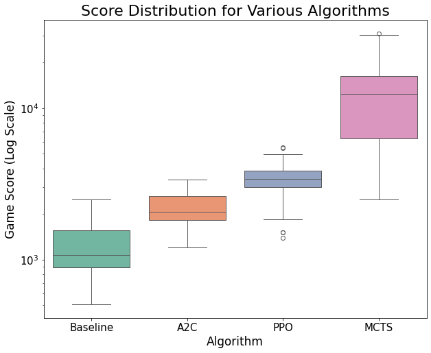
An ANOVA test shows that there is a significant difference in the mean game scores across models, p < 0.0001. Specifically, a post-hoc Tukey’s HSD test shows that MCTS performs significantly better on average than the baseline (p < 0.0001), PPO (p < 0.0001), and A2C (p < 0.0001). Although the PPO and A2C models appeared to outperform the baseline, these differences were not statistically significant (p = 0.08 and p = 0.69, respectively). With a mean score of 12,592, it is clear that MCTS is dominant in this game compared to the other models that we tested.
In terms of the highest tile reached, only MCTS was ever able to reach the 2048 tile. This occurred in 3 out of the 30 games, or 10% of the time. This greatly exceeds our original goal of 5%. Because of the massive state space and randomness of this task, we consider this model to be fairly successful. The results we achieved are similar to the 11% win rate achieved by a previous study using an MCTS model with a comparable number of rollouts [1].
Algorithm Speed
Speed is not crucial to the 2048 game itself, as there is no time limit in any standard implementation of the game. However, it does serve as an important comparison of efficiency which may be a key factor for other similar reinforcement learning tasks. The plot below shows the number of moves made over time by each of the models. Time beyond 80 seconds is not shown, as the baseline, PPO, and A2C models would reach the ‘game over’ state before this.
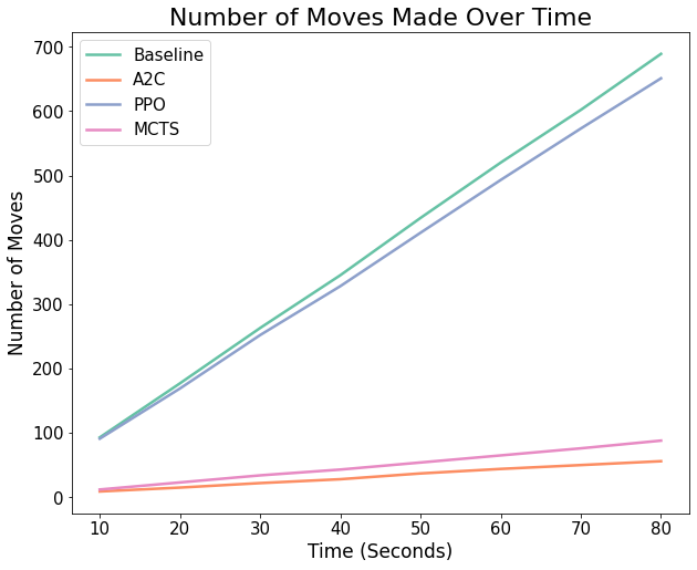
We see that PPO performs moves extremely quickly, and almost reaches the speed of the baseline which is selecting random moves. This made it very efficient for repeated testing and hyperparameter optimization, but in the case of 2048, the speed was not beneficial as the model did not get very far in the game. A2C and MCTS perform relatively similarly in terms of speed, taking much longer to make each move. For MCTS, this was caused by the algorithm perfoming many rollouts in order to find the next best move, and increasing the rollouts to even larger values results in significantly slowed gameplay. However, because this approach proves to be successful, the slower speed is a worthy cost for 2048. This may not be the case for other similar tasks. For A2C, the continuous training of both the actor and critic neural network resulted in a gameplay that is slightly slower than even MCTS.
Summary and Takeaways
In our proposal, we stated that we would explore and compare the efficacy of various reinforcement learning algorithms in playing the game 2048.
We can confidently say that A2C does not seem to be well-suited for this game. When compared to the other two RL models - one of which is also a Policy Gradient Algorithm like A2C - it was both the slowest and worst performing. The potential reasons for this are discussed in the A2C portion of the Approaches section of this report. In summary, its focus on learning by experience rather than planning paired with its sensitivity to hyperparameters makes A2C underperform in comparison to the efficacy of other RL algorithms. While it is able to consistently surpass the baseline, the hugely slower speed of this algorithm makes even that accomplishment irrelevant in some environments.
PPO, on the other hand, showed potential. With more time, we would like to investigate more methods to improve the PPO model as it showed decent performance possibilities and unmatched speed, which can be very beneficial in other game environments. In the case of 2048, however, it barely surpasses A2C and comes no where near the achievement of MCTS.
MCTS is the clear winner of our analysis due to its unmatched ability to actually hit the 2048 tile. As stated in the Game Performance section above, the capabilities of this model have doubled our original goal of hitting 2048 at a rate of 5%.
All that in mind, we rank our models on their ability to successfully play the game of 2048 as follows:
- MCTS: slow, scores ~12500 on average, and the only model to successfully reach 2048 (10% of the time)
- PPO: fast, scores ~3500 on average
- A2C: slow, scores ~2000 on average
- Baseline: makes random moves, scores ~1200 on average
In the future, we would find it interesting to implement more algorithms - perhaps including some that are not in the category of RL - to continue to evaluate what types of machine learning agents are suited for the suprisingly complex task of solving 2048.
References
Libraries:
- General Python Libraries: concurrent, copy, json, os, Pygame, random, sys
- AI/ML/Computing Libraries: Keras, Matplotlib, NumPy, TensorFlow
2048 in Python:
- Game Logic/Rendering (game_logic.py, game_renderer.py): https://github.com/scar17off/ai-2048
- 2048 Python Game Simulation (run_simulation.py): Modified version of the original file “ai_play.py” in https://github.com/scar17off/ai-2048/tree/main
Algorithm Implementation Approaches:
- Monte Carlo Tree Search (MCTS) approach (mcts.py): inspired by the implementation for Tic-Tac-Toe at https://www.stephendiehl.com/posts/mtcs/
- Proximal Policy Optimization (PPO) approach (ppo.py): inspired by the implementation of PPO at https://iclr-blog-track.github.io/2022/03/25/ppo-implementation-details/
- Advantage Actor-Critic (A2C) approach (a2c.py): inspired by the implementation for CartPole at https://www.geeksforgeeks.org/actor-critic-algorithm-in-reinforcement-learning/
Referenced Papers and Resources:
- [1] Goenawan, N., Tao, S., Wu, K. “What’s in a Game: Solving 2048 with Reinforcement Learning”. https://web.stanford.edu/class/aa228/reports/2020/final41.pdf
- [2] https://github.com/haakon8855/mcts-reinforcement-learning
- [3] https://github.com/hsiehjackson/Deep-Reinforcement-Learning-on-Atari-Games
- [4] https://njustesen.github.io/botbowl/a2c.html
- [5] Guei, H. “On Reinforcement Learning for the Game of 2048”. https://arxiv.org/abs/2212.11087
- [6] https://www.chessprogramming.org/UCT
- [7] https://blogs.oracle.com/ai-and-datascience/post/reinforcement-learning-q-learning-made-simple
- [8] https://medium.com/@dixitaniket76/advantage-actor-critic-a2c-algorithm-explained-and-implemented-in-pytorch-dc3354b60b50
- [9] https://www.geeksforgeeks.org/actor-critic-algorithm-in-reinforcement-learning/
- [10] https://schneppat.com/advantage-actor-critic_a2c.html
- [11] https://iclr-blog-track.github.io/2022/03/25/ppo-implementation-details/
AI Tool Usage
- Used ChatGPT in line with other online resources to gain a better understanding of the algorithms before implementation (i.e. had the chatbot summarize, give use case examples, etc.)
- Used ChatGPT to aid in the fixing of minor bugs during implementation process